Hazards of hazard ratios

Causal inference series

Michael C Sachs

Quick review of survival analysis

Defining features of survival data

• A continuous time variable
  • Research interest is on the length of time elapsing between two events.
  • Time from diagnosis to event = length of follow up
• A binary event variable
  • Indicates whether the event of interest occurred (1 = yes, 0 = no)
  • If 1, the time is the time at which the event occurred
  • If 0, the last follow-up time = censored
  • Censored means that the event occurs after the recorded follow-up time
    • Possibly useful information!

The survival function

• Definition: \(S(t) = P(T > t) =\) probability that the event of interest occurs after time \(t\)
• Properties
  • \(0 \leq S(t) \leq 1\) because \(S(t)\) is a probability.
  • \(S(0) = 1\) because everyone is event-free at baseline.
  • \(S(b) \leq S(a)\) if \(a \leq b\). The survival probability does not increase with time.

Information in the survival function

• The \(S(t)\) curve contains all information on how the survival probability changes over time
• We can use it to compute:
  • The 1-year survival probability
  • Survival quantiles (e.g., median)
  • The mean survival

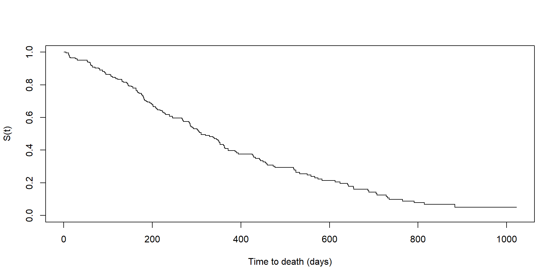
Example (lung cancer data)

The hazard function

Definition:

• \(h(t)\) = instantaneous rate of death at time \(t\)
• The probability of death per time-unit at \(t\), among those who survived until just before \(t\)
• \(h(t) = \lim_{\delta \rightarrow 0} \frac{P(t \leq T < t + \delta | T \geq t)}{\delta}.\)

Properties:

• \(h(t) = -(d/dt S(t))/(S(t)) = f(t) / S(t)\) where \(f(t)\) is the probability density function
• \(S(t) = \exp(-\int_0^t h(x) \, dx)\)
• Range: \([0, \infty)\)
• Is related to survival function, but different scale
• Not a probability, a rate

Basic Cox proportional hazards model (Cox, D.R., 1972, JRSS-B)

For a covariate \(x\), the basic Cox model assumes

\[h(t | x) = h_0(t) \exp(\beta_1 \cdot x)\]

where \(h_0(t)\) is the baseline hazard function.

Assumption: Proportional hazards (PH).

• The hazard function for any covariate value \(x\) is proportional to the baseline hazard \(h_0(t)\)
• The multiplicative factor is called the hazard ratio, which does not depend on time \(t\)
• The coefficient \(\beta_1\) is called the log hazard ratio.

\[ \frac{h(t | x = 1)}{h(t | x = 0)} = \frac{h_0(t) \exp(\beta_1 \cdot 1)}{h_0(t) \exp(\beta_1 \cdot 0)} = \exp(\beta_1) \]

The baseline hazard

\[h(t | x = 0) = h_0(t) \exp(\beta_1 \cdot 0) = h_0(t).\]

• \(h_0(t)\) is the hazard function for the stratum with exposure = 0.
  • This does depend on time
  • We make no assumptions on what the shape of the function is: it is a semi-parametric model

In his own words

“The present paper is largely concerned with the extension of the results of Kaplan and Meier to the … incorporation of regression-like arguments into life-table analysis.”

“A simple form for the hazard is not by itself particularly advantageous, and models other than [Cox’s] may be more natural.”

“In the present paper we shall, however, concentrate on exploring the consequence of allowing \(h_0(t)\) to be arbitrary, main interest being in the regression parameters”

Cox, D. R. Regression models and life tables, J. R. Stat. Soc. B 34, 187–220 (1972).

About 50,000 citations.

Why is the Cox model so popular?

• Easy to use, available in all stats software packages
• Computationally nice, rarely fails or gives warnings
• Simple – it reduces something complex to a single number
• Theoretically interesting for statisticians – the Cox partial likelihood led to new theoretical development in the field (e.g. PK Andersen’s work)

Causal inference

• Causal effects can be thought of as the change in the summary statistic of an outcome variable associated with the manipulation of an exposure variable from/to a particular level.
• We have observations, which are usually generated via mechanisms that do not involve manipulation of the exposure.
• The goal is to use the distribution of the observations to inform us about the causal effect of interest

DAGs and observations

A directed acyclic graph (or DAG or just graph) conveys our assumptions about the mechanisms that gave rise to the observations, e.g.,

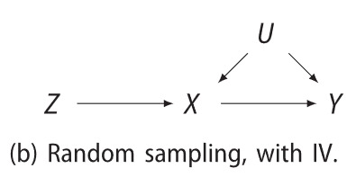
This is a functional causal model \(\{F_V:pa(V)\times U_V\to V\mid V\in\mathcal{V}\}\), e.g., \(y = F_Y(x, u, \varepsilon_Y)\).

Effects

A causal effects will be written as e.g., \(p\{Y(X = 1) = 1\} - p\{Y(X = 0) = 1\}\), where \(Y(X = 1)\) is the potential outcome which means

“the variable \(Y\) if \(X\) were intervened upon to have value 1”.

Back to hazard ratios

• We often are interested the causal effect on a time-to-event outcome with right censoring in our study (examples?)
• The flow-chart approach to statistics tells us that we should use the Cox model in this situation, which gives us the hazard ratio (maybe adjusted for confounders), which we interpret as our estimated causal effect.

What are the two problems that Hernán points out in this situation?

The problems

1. The real hazard ratios probably depend on time
2. Built-in selection bias

Both problems lead to difficulties in interpreting the HR as a causal effect (unless it equals 1)

Illustration (by Torben Martinussen)

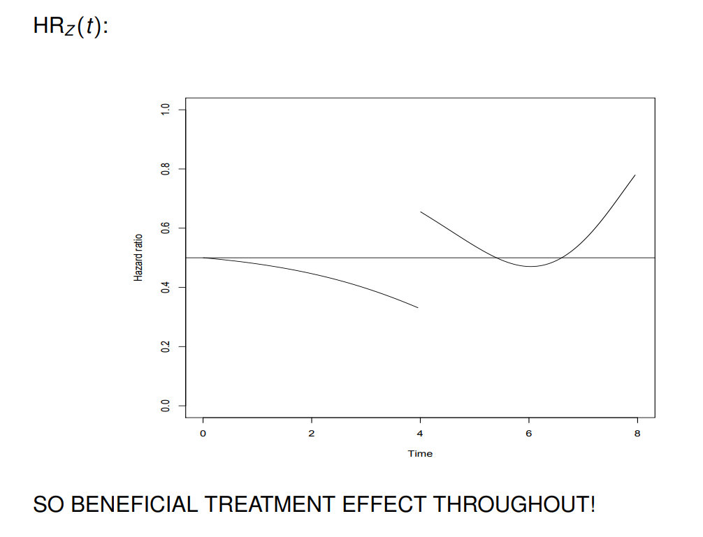
Suppose \[ \lambda(t;X)=\{e^{\beta_1X}I(t\leq 4)+ e^{\beta_2X}I(t>4)\} \lambda_0(t) \] is the true hazard. One HR on \([0,4]\) (beneficial on this range) and another one on \((4,\tau [\) (no effect on this range).

Let’s also assume that we are in a randomized trial, so no variables impact the treatment assignment.

Is it possible that other variables may impact survival time? Yes!

Frailty

Frailty is the term for a random effect that affects survival, in our model we may have

\[ \lambda(t;X,Z)=Z\lambda^*(t;X) \]

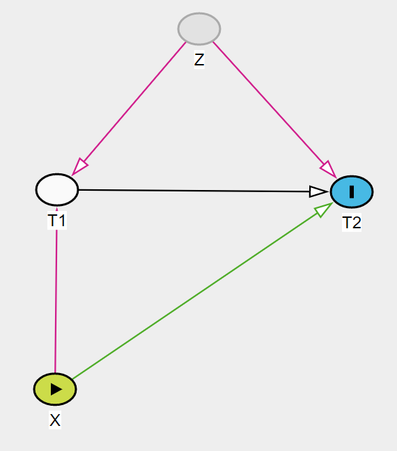
where \(Z\) is a random variable with mean and variance 1. In this case we can derive the HR as a function of \(Z\), which is closer to a causal effect (see DAG in next slide)

Effect given \(Z\)

DAG in this setting

Summary

Keep in mind that we do not obtain biased estimates, but arguing about the treatment effect using the hazard ratio simply leads to a wrong conclusion

• Exchangeability due to randomization only holds at time \(t=0\), it is lost when \(t>0\).
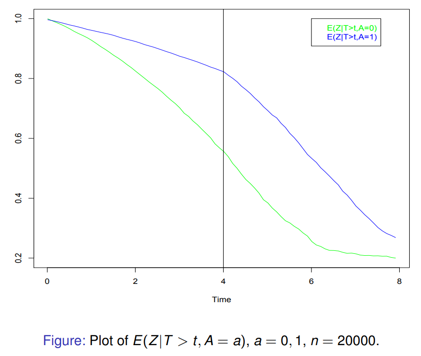
• We have, for \(t\le v\), that \[ E(Z|T>t,X=x)= \left\{ \begin{array}{ll} \exp{\{-\Lambda_0(t)\}} & \textrm{if $x=0$}\\ \exp{\{-\Lambda_0(t)e^{\beta_1}\}} & \textrm{if $x=1$}\\ \end{array} \right. \] so indeed selection is taking place: \[ E(Z|T>t,X=1)>E(Z|T>t,X=0). \]

Frailty selection

Solutions

What do? What does Hernán suggest?

Use “cumulative” estimands, that have nice causal interpretations, e.g.,

Differences or ratios in survival probabilities at fixed times: \(P(T > t | X = 1) - P(T > t | X = 0)\)

Differences or ratios in restricted mean survival.

Practicalities

IPTW survival curves to adjust for confounding (how to do inference?)

More options:

• stdReg R package, to do standardization to adjust for covariate while estimating survival probabilities
• eventglm R package, regression modeling of survival probabilities and restricted mean survival
• timereg R package, direct modeling of the same
• Accelerated failure time models, which directly model effects on survival (see reference 5)

Questions?