Run the Shiny application like so. The result is assigned to an
objected called results so that you can save the results
that are produced in the web interface.
results <- specify_graph()A new window in your system’s default web browser is opened with the following interface:
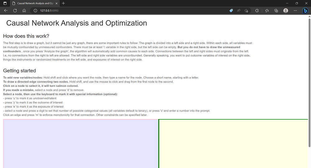
The instructions at the top provide details on how to specify the graph. The graph is divided into a left side and a right side. There is no confounding allowed between the left and right sides. All variables on the right side are confounded. Connections between the left and right sides must originate from the left. I.e, no connections from the right to left are allowed. On the left side, arbitrary connections are allowed and the model assumes that all nodes are observed and connected. On the right side, unmeasured variables are allowed, and the procedure assumes unmeasured confounding between all nodes. These restrictions ensure that the problem can be solved analytically using linear optimization.
In the main window below the text, Shift+click to add nodes. When a node is added, you are prompted to give it a name. Make sure that you use a valid R variable name, but without underscores. This means it cannot start with a number, and cannot contain spaces, underscores or special characters. Single capital letters are good choices, possibly with trailing numbers.
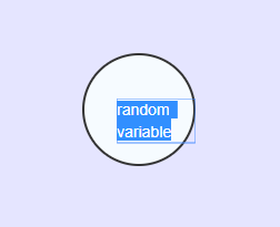
Click on an existing node to select it, and shift+click on a node to change the name. Shift+drag to connect nodes. Remember than no edges may go from the right side to the left side. Click a node to select and then press ‘u’ to mark it as unobserved/latent. Select a node and press a digit to set that number of possible categorical values (all variables default to binary), or press ‘c’ and enter a number into the prompt. Click to select nodes/edges and press ‘d’ to remove. If there are problems selecting nodes, try restarting your browser.
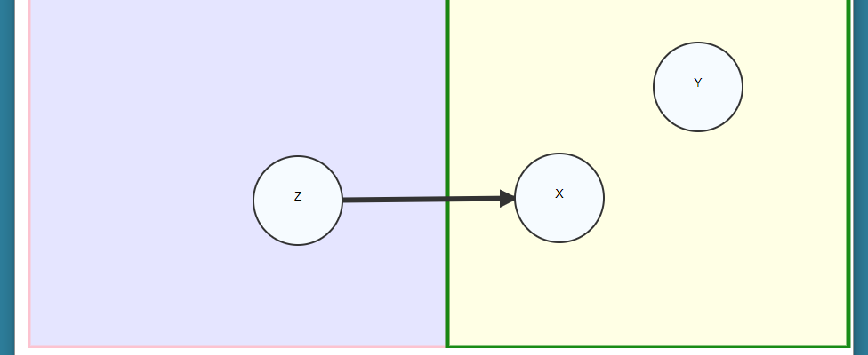
Once we have our graph specified, we can optionally make some annotations. You may specify the outcome of interest, and the exposure of interest. Select the outcome node and press ‘y’ to mark it as the outcome of interest, and then select the exposure node and press ‘e’ to mark it as the exposure of interest. The default causal contrast is the total effect. The exposure will be colored blue, and the outcome colored red.
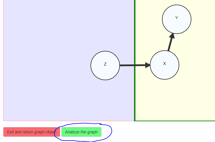
We now have a graph specified that is ready to be analyzed.
Optionally, click an edge and press ‘m’ to enforce monotonicity for that
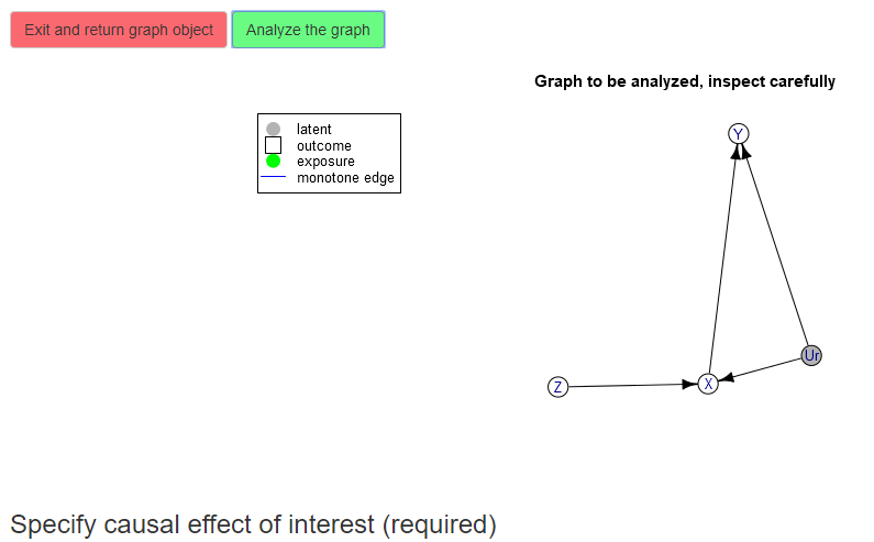
connection. If you are ready to analyze the object click on the “Press
to analyze the graph button”. The program interprets the graph, converts
it to an igraph object with annotations, and prints the
result from R. Inspect the resulting graph carefully so that you
understand what is being analyzed. Note that if a side contains at least
two variables then a confounder has been automatically added for
them.
Specifying the causal effect of interest
The next step is to use the text box to specify the causal effect of interest. In our current example, we are interested in the causal risk difference in Y comparing X = 1 to X = 0, i.e., Y(X = 1) - Y(X = 0). The optimizer will compute bounds for the expected value of this quantity.
Use the text box to describe your causal effect of interest. The effects must be of the form
p{V11(X=a)=a; V12(X=a)=b;...} op1 p{V21(X=b)=a; V22(X=c)=b;...} op2 ...where Vij are names of variables in the graph,
a, b are corresponding values, and op are
either - or +. You can specify a single
probability statement (i.e., no operator). Note that the probability
statements begin with little p, and use curly braces, and items inside
the probability statements are separated by ;. The
variables may be potential outcomes which are denoted by parentheses.
Variables may also be nested inside potential outcomes. Pure
observations such as p{Y = 1} are not allowed if the left
side contains any variables. If the left side contains any variables,
then they mush be ancestors of the intervention set variables (or the
intervention variables themselves). All of the following are valid
effect statements:
p{Y(X = 1) = 1} - p{Y(X = 0) = 1}
p{X(Z = 1) = 1; X(Z = 0) = 0}
p{Y(M(X = 0), X = 1) = 1} - p{Y(M(X = 0), X = 0) = 1}
Back to our example, we specify the effect as
p{Y(X = 1) = 1} - p{Y(X = 0) = 1}then click the “parse” button to fix the effect.
Specifying constraints (optional)
Once the causal effect of interest has been specified, you may optionally specify some constraints. Click the button to start the constraint interface.
Here you can specify potential outcomes to constrain by writing the potential outcomes, values of their parents, and operators that determine the constraint (equalities or inequalities). In our example, we can specify monotonicity of the instrument Z by defining the constraint X(Z = 1) X(Z = 0):
X(Z = 1) >= X(Z = 0)then click parse.
Computation of the bounds
Once you have inspected the graph, specified the causal effect, and understand what is being analyzed, press the final button to compute the bounds.
Note that the computation may take a significant amount of time.
The results are summarized in plain text. The bounds are expressed as
the minimum/maximum of a series of expressions involving the conditional
probabilities of the observed variables. For more details on the method
see this
paper. The final button allows you to return all of the objects back
to the R environment and store them in results.
The results object contains the graph, the
parameterization and interpretation of the graph in terms of the
variables and parameters, the bounds and log information about the
optimization procedure, and an R function that implements the
bounds:
names(results)
#> [1] "graphres"       "obj"            "bounds.obs"     "constraints"
#> [5] "effect"         "boundsFunction"

print(results$bounds.obs)
#> lower bound =
#> MAX {
#>   p00_0 - p00_1 - p10_1 - p01_1
#> }
#> ----------------------------------------
#> upper bound =
#> MIN {
#>   1 - p10_1 - p01_0
#> }
#>
#> A function to compute the bounds for a given set of probabilities is available in the x$bounds_function element.

print(results$boundsFunction)
#> function (p00_0 = NULL, p00_1 = NULL, p10_0 = NULL, p10_1 = NULL,
#>     p01_0 = NULL, p01_1 = NULL, p11_0 = NULL, p11_1 = NULL)
#> {
#>     lb <- pmax(p00_0 - p00_1 - p10_1 - p01_1)
#>     ub <- pmin(1 - p10_1 - p01_0)
#>     if (any(ub < lb)) {
#>         warning("Invalid bounds! Data probably does not satisfy the assumptions in the DAG!")
#>     }
#>     data.frame(lower = lb, upper = ub)
#> }
The results object can also be used to numerically simulate the
bounds. Try using the simulate_bounds function.
sim <- simulate_bounds(results$obj, results$bounds.obs, nsim = 100)
head(sim)
#>     objective bound.lower bound.upper
#> 1  0.11072239  -0.2765626   0.4145571
#> 2  0.04677063  -0.3380446   0.4131181
#> 3 -0.20689850  -0.4887614   0.1605880
#> 4  0.14317449  -0.2369513   0.3885858
#> 5  0.02464152  -0.3451034   0.3450640
#> 6  0.09175714  -0.2020024   0.3795258
We also provide a helper function to print the bounds as latex
equations. Use the latex_bounds function.
cat(latex_bounds(results$bounds.obs$bounds, results$obj$parameters))Please sends any bugs or feedback to sachsmc@gmail.com or file an issue on https://github.com/sachsmc/causaloptim .