Multiple causes and times

Learning objectives

In this lesson you will

1. Fit and understand basic models for competing risks settings
2. Fit and understand basic joint models for multiple time points of interest
3. Compare and contrast the eventglm models with cloglog link to Cox regression models

Setup

Library the survival package and then the eventglm package. We will use some commands from survival to make sense of what is going on in the regression models.

library(survival)
library(eventglm)

Monoclonal gammopathy data (Competing risks)

Our next example involves the mgus2 dataset, included in the package:

## ?mgus2
head(mgus2)

##   id age sex dxyr  hgb creat mspike ptime pstat futime death etime event
## 1  1  88   F 1981 13.1   1.3    0.5    30     0     30     1    30 death
## 2  2  78   F 1968 11.5   1.2    2.0    25     0     25     1    25 death
## 3  3  94   M 1980 10.5   1.5    2.6    46     0     46     1    46 death
## 4  4  68   M 1977 15.2   1.2    1.2    92     0     92     1    92 death
## 5  5  90   F 1973 10.7   0.8    1.0     8     0      8     1     8 death
## 6  6  90   M 1990 12.9   1.0    0.5     4     0      4     1     4 death

This dataset has a number of covariates, and the time until progression to plasma cell malignancy (PCM), or death. Here the event PCM is of primary interest, with death being a competing event. The data are described and analyzed in the survival vignette (section 2.3.2):

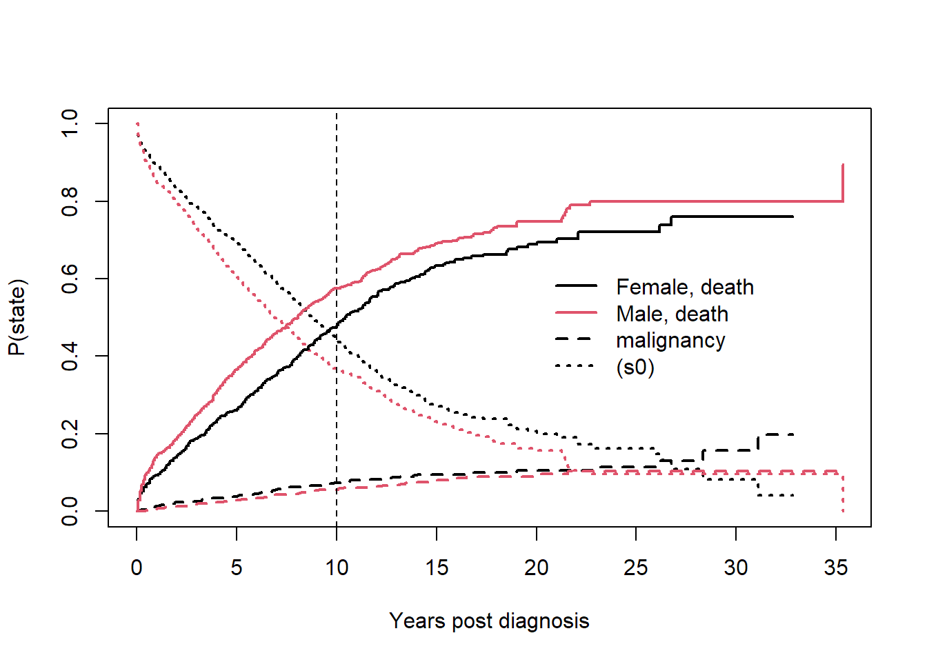
crfit <- survfit(Surv(etime, event) ~ sex, eventglm::mgus2)
summary(crfit, times = 120)

## Call: survfit(formula = Surv(etime, event) ~ sex, data = eventglm::mgus2)
## 
##                 sex=F 
##     time   n.risk  n.event  P((s0))   P(pcm) P(death) 
## 120.0000 214.0000 331.0000   0.4456   0.0739   0.4805 
## 
##                 sex=M 
##     time   n.risk  n.event  P((s0))   P(pcm) P(death) 
## 120.0000 210.0000 450.0000   0.3695   0.0553   0.5752

print(crfit, rmean = 120)

## Call: survfit(formula = Surv(etime, event) ~ sex, data = eventglm::mgus2)
## 
##                n nevent    rmean*
## sex=F, (s0)  631      0 82.983485
## sex=M, (s0)  753      0 74.808346
## sex=F, pcm   631     59  4.794595
## sex=M, pcm   753     56  3.501305
## sex=F, death 631    370 32.221921
## sex=M, death 753    490 41.690349
##    *mean time in state, restricted (max time = 120 )

plot(crfit, col=1:2,  noplot="",
     lty=c(3,3,2,2,1,1), lwd=2, xscale=12,
     xlab="Years post diagnosis", ylab="P(state)")
legend(240, .65, c("Female, death", "Male, death", "malignancy", "(s0)"),
       lty=c(1,1,2,3), col=c(1,2,1,1), bty='n', lwd=2)
abline(v = 120, lty = 2)

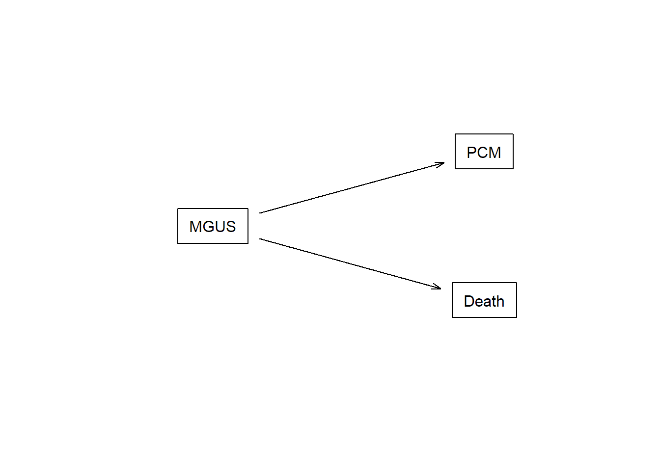
This is the competing risks setting, which can be described with the multi-state model in the figure below.

connect <- matrix(0, nrow = 3, ncol = 3, 
                  dimnames = lapply(1:2, \(i) c("MGUS", "PCM", "Death")))
connect[1, 2:3] <- 1
statefig(c(1, 2), connect)

We can get similar estimates for the cumulative incidence of pcm at 10 years and the expected lifetime lost due to pcm up to 10 years with similar commands as above. Note the cause option to specify the cause of interest.

mgfitci <- cumincglm(Surv(etime, event) ~ sex, cause = "pcm", 
                     time = 120, data = mgus2)
summary(mgfitci)

## 
## Call:
## cumincglm(formula = Surv(etime, event) ~ sex, time = 120, cause = "pcm", 
##     data = mgus2)
## 
## Deviance Residuals: 
##      Min        1Q    Median        3Q       Max  
## -0.08163  -0.07447  -0.06306  -0.05536   1.23923  
## 
## Coefficients:
##             Estimate Std. Error z value Pr(>|z|)    
## (Intercept)  0.07383    0.01086   6.800 1.04e-11 ***
## sexM        -0.01857    0.01384  -1.342     0.18    
## ---
## Signif. codes:  0 '***' 0.001 '**' 0.01 '*' 0.05 '.' 0.1 ' ' 1
## 
## (Dispersion parameter for quasi family taken to be 1)
## 
##     Null deviance: 88.507  on 1383  degrees of freedom
## Residual deviance: 88.388  on 1382  degrees of freedom
## AIC: NA
## 
## Number of Fisher Scoring iterations: 2

mgfitrmean <- rmeanglm(Surv(etime, event) ~ sex, cause = "pcm", 
                       time = 120, data = mgus2)
summary(mgfitrmean)

## 
## Call:
## rmeanglm(formula = Surv(etime, event) ~ sex, time = 120, cause = "pcm", 
##     data = mgus2)
## 
## Deviance Residuals: 
##     Min       1Q   Median       3Q      Max  
##  -4.971   -4.863   -3.678   -3.508  113.292  
## 
## Coefficients:
##             Estimate Std. Error z value Pr(>|z|)    
## (Intercept)   4.7926     0.7883   6.080  1.2e-09 ***
## sexM         -1.2929     0.9902  -1.306    0.192    
## ---
## Signif. codes:  0 '***' 0.001 '**' 0.01 '*' 0.05 '.' 0.1 ' ' 1
## 
## (Dispersion parameter for quasi family taken to be 1)
## 
##     Null deviance: 450225  on 1383  degrees of freedom
## Residual deviance: 449652  on 1382  degrees of freedom
## AIC: NA
## 
## Number of Fisher Scoring iterations: 2

This time the models are \[ P(T \leq 120 \mbox{ and } \delta = \mbox{PCM} | \mbox{sex}) = \beta_0 + \beta_1 I(sex = "M") \] for the cause specific cumulative incidence, and \[ E((120 - T \wedge 120)I(\delta = \mbox{PCM}) | \mbox{sex}) = \beta_0 + \beta_1 I(sex = "M") \] for the second model. The latter is interpreted as the expected lifetime lost due to PCM up to 120 months. See Andersen (2013) for more details on this quantity.

Exercise

Look at the mgus2 dataset, summarize the variables in the data, and read the help file for mgus2 in the eventglm documentation. Then specify and fit a regression model to answer a particular scientific question for this dataset. Interpret the relevant coefficients from the model.

Solution

summary(mgus2)

##        id              age        sex          dxyr           hgb      
##  Min.   :   1.0   Min.   :24.00   F:631   Min.   :1960   Min.   : 5.7  
##  1st Qu.: 346.8   1st Qu.:63.00   M:753   1st Qu.:1980   1st Qu.:12.2  
##  Median : 692.5   Median :72.00           Median :1984   Median :13.5  
##  Mean   : 692.5   Mean   :70.42           Mean   :1983   Mean   :13.3  
##  3rd Qu.:1038.2   3rd Qu.:79.00           3rd Qu.:1988   3rd Qu.:14.7  
##  Max.   :1384.0   Max.   :96.00           Max.   :1994   Max.   :18.9  
##                                                          NA's   :13    
##      creat            mspike          ptime            pstat        
##  Min.   : 0.400   Min.   :0.000   Min.   :  1.00   Min.   :0.00000  
##  1st Qu.: 0.900   1st Qu.:0.600   1st Qu.: 37.00   1st Qu.:0.00000  
##  Median : 1.100   Median :1.200   Median : 81.00   Median :0.00000  
##  Mean   : 1.292   Mean   :1.164   Mean   : 93.54   Mean   :0.08309  
##  3rd Qu.: 1.300   3rd Qu.:1.500   3rd Qu.:136.25   3rd Qu.:0.00000  
##  Max.   :22.000   Max.   :3.000   Max.   :424.00   Max.   :1.00000  
##  NA's   :30       NA's   :11                                        
##      futime          death            etime           event    
##  Min.   :  1.0   Min.   :0.0000   Min.   :  1.00   censor:409  
##  1st Qu.: 40.0   1st Qu.:0.0000   1st Qu.: 37.00   pcm   :115  
##  Median : 84.0   Median :1.0000   Median : 81.00   death :860  
##  Mean   : 95.8   Mean   :0.6958   Mean   : 93.54               
##  3rd Qu.:139.0   3rd Qu.:1.0000   3rd Qu.:136.25               
##  Max.   :424.0   Max.   :1.0000   Max.   :424.00               
## 

The purpose of this study was to determine whether there are any reliable predictors of progression to malignancy.

mgfitci2 <- cumincglm(Surv(etime, event) ~ sex + age + hgb + creat + mspike, 
                      cause = "pcm", 
                      time = 120, data = mgus2)
summary(mgfitci2)

## 
## Call:
## cumincglm(formula = Surv(etime, event) ~ sex + age + hgb + creat + 
##     mspike, time = 120, cause = "pcm", data = mgus2)
## 
## Deviance Residuals: 
##      Min        1Q    Median        3Q       Max  
## -0.18803  -0.08596  -0.06097  -0.03109   1.19792  
## 
## Coefficients:
##               Estimate Std. Error z value Pr(>|z|)    
## (Intercept)  3.930e-02  6.295e-02   0.624  0.53238    
## sexM        -1.443e-02  1.417e-02  -1.019  0.30841    
## age         -3.672e-05  4.500e-04  -0.082  0.93496    
## hgb         -1.554e-03  3.516e-03  -0.442  0.65840    
## creat       -7.625e-03  2.878e-03  -2.649  0.00807 ** 
## mspike       5.685e-02  1.427e-02   3.983 6.81e-05 ***
## ---
## Signif. codes:  0 '***' 0.001 '**' 0.01 '*' 0.05 '.' 0.1 ' ' 1
## 
## (Dispersion parameter for quasi family taken to be 1)
## 
##     Null deviance: 86.385  on 1337  degrees of freedom
## Residual deviance: 84.738  on 1332  degrees of freedom
##   (46 observations deleted due to missingness)
## AIC: NA
## 
## Number of Fisher Scoring iterations: 2

mgfitrmean2 <- rmeanglm(Surv(etime, event) ~ sex + age + hgb + creat + mspike, 
                        cause = "pcm", 
                      time = 120, data = mgus2)
summary(mgfitrmean2)

## 
## Call:
## rmeanglm(formula = Surv(etime, event) ~ sex + age + hgb + creat + 
##     mspike, time = 120, cause = "pcm", data = mgus2)
## 
## Deviance Residuals: 
##     Min       1Q   Median       3Q      Max  
## -13.738   -5.580   -3.688   -1.748  111.199  
## 
## Coefficients:
##             Estimate Std. Error z value Pr(>|z|)    
## (Intercept)  1.40587    4.45719   0.315 0.752446    
## sexM        -0.87102    0.99635  -0.874 0.382005    
## age          0.03851    0.03034   1.269 0.204405    
## hgb         -0.27601    0.27655  -0.998 0.318256    
## creat       -0.41408    0.21143  -1.958 0.050176 .  
## mspike       4.03216    1.10280   3.656 0.000256 ***
## ---
## Signif. codes:  0 '***' 0.001 '**' 0.01 '*' 0.05 '.' 0.1 ' ' 1
## 
## (Dispersion parameter for quasi family taken to be 1)
## 
##     Null deviance: 438200  on 1337  degrees of freedom
## Residual deviance: 429463  on 1332  degrees of freedom
##   (46 observations deleted due to missingness)
## AIC: NA
## 
## Number of Fisher Scoring iterations: 2

The size of the monoclonal serum spike appears to be an independent predictor of the risk of pcm within 10 years, with a 5.7% higher risk for each unit increase in mspike, adjusted for creatinine, hemoglobin, age and sex. Likewise, a unit increase in mspike is associated with an expected 4 months lifetime lost due to PCM, adjusted for the other variables.

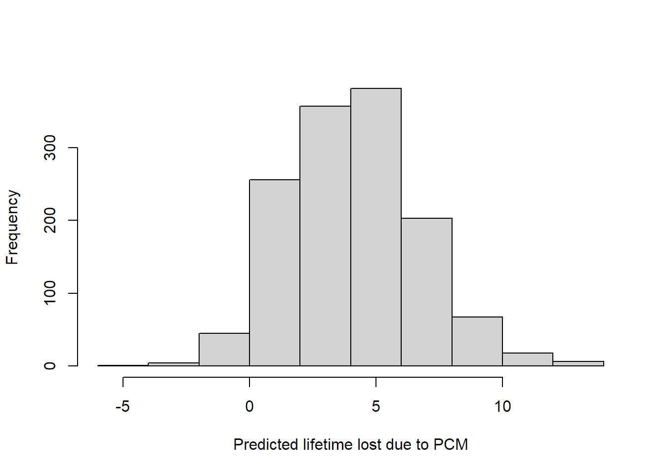
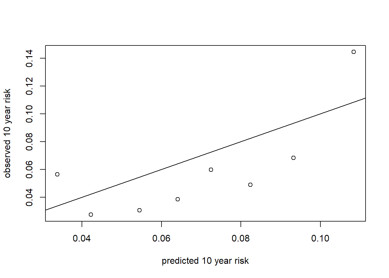
The objects returned by cumincglm and rmeanglm inherit from glm, so many methods are available, including predict and resid. Residuals use the scaling factor suggested by Perme and Andersen (2008), as do predictions. Predicted restricted means give a possible method to predict individual event times, while the predicted cumulative incidence should be probabilities. Note that with the identity link, the predicted cumulative incidence is not guaranteed to be between 0 and 1.

hist(predict(mgfitrmean2, newdata = mgus2), 
     xlab = "Predicted lifetime lost due to PCM", main = "")

mgus2$prob.pcm10 <- predict(mgfitci2, newdata = mgus2)
mgus2$pseudo.ci <- mgfitci$y
summary(mgus2$prob.pcm10)

##     Min.  1st Qu.   Median     Mean  3rd Qu.     Max.     NA's 
## -0.09178  0.03774  0.06411  0.06423  0.08706  0.18443       46

cutps <- quantile(mgus2$prob.pcm10, seq(.1, .9, by = .1), na.rm = TRUE)
mgus2$prob.cut <- cut(mgus2$prob.pcm10, 
                      cutps)
pred.p <- cutps[-length(cutps)] + diff(cutps)
obs.p <- c(by(mgus2$pseudo.ci, mgus2$prob.cut, mean))
plot(obs.p ~ pred.p, xlab = "predicted 10 year risk", ylab = "observed 10 year risk")
abline(0, 1)

Joint modelling over multiple times

You can specify a vector of times in cumincglm to get a model that assumes the effect of the covariate is constant over those times. Let’s see how this works in the colon example.

mvtfit1 <- cumincglm(Surv(time, status) ~ rx, 
        time = c(500, 1000, 1500, 2000, 2500),
        data = colon, survival = TRUE)
summary(mvtfit1)

## 
## Call:
## cumincglm(formula = Surv(time, status) ~ rx, time = c(500, 1000, 
##     1500, 2000, 2500), data = colon, survival = TRUE)
## 
## Deviance Residuals: 
##    Min      1Q  Median      3Q     Max  
##                                         
## 
## Coefficients:
##                          Estimate Std. Error z value Pr(>|z|)    
## (Intercept)              0.829127   0.021793  38.046  < 2e-16 ***
## factor(pseudo.time)1000 -0.170283   0.012340 -13.800  < 2e-16 ***
## factor(pseudo.time)1500 -0.263039   0.014456 -18.196  < 2e-16 ***
## factor(pseudo.time)2000 -0.314852   0.015290 -20.592  < 2e-16 ***
## factor(pseudo.time)2500 -0.351750   0.016423 -21.419  < 2e-16 ***
## rxLev                    0.003942   0.032530   0.121  0.90355    
## rxLev+5FU                0.093737   0.031979   2.931  0.00338 ** 
## ---
## Signif. codes:  0 '***' 0.001 '**' 0.01 '*' 0.05 '.' 0.1 ' ' 1
## 
## (Dispersion parameter for quasi family taken to be 1)
## 
##     Null deviance: 1091.5  on 4644  degrees of freedom
## Residual deviance: 1009.4  on 4638  degrees of freedom
## AIC: NA
## 
## Number of Fisher Scoring iterations: 2

This fits the model (in general terms) \[g\{P(T_i < t_b| X_i = x_i)\} = (\beta_0 + \beta_b) + \beta_1x_i, b = 1, \ldots, k.\]

In this model, the intercept is the survival probability in the Obs arm at time 500 (the reference time). The terms labeled factor(pseudo.time)t represent the change in the intercept associated with the time t. So, for example, the survival probability in the Obs arm at time 1000 is 0.83 + -0.17 = 0.66.

Looking at the survival curves in previous lesson, the assumption of a constant treatment effect on the survival difference scale may be questionable. We can allow covariate effects to be time dependent by wrapping them in the special term tve() in the right side of the formula.

mvtfit2 <- cumincglm(Surv(time, status) ~ tve(rx), 
        time = c(500, 1000, 1500, 2000, 2500),
        data = colon, survival = TRUE)
summary(mvtfit2)

## 
## Call:
## cumincglm(formula = Surv(time, status) ~ tve(rx), time = c(500, 
##     1000, 1500, 2000, 2500), data = colon, survival = TRUE)
## 
## Deviance Residuals: 
##    Min      1Q  Median      3Q     Max  
##                                         
## 
## Coefficients:
##                                    Estimate Std. Error z value Pr(>|z|)    
## (Intercept)                        0.850710   0.020078  42.370  < 2e-16 ***
## factor(pseudo.time)1000           -0.178401   0.021560  -8.275  < 2e-16 ***
## factor(pseudo.time)1500           -0.289898   0.025561 -11.341  < 2e-16 ***
## factor(pseudo.time)2000           -0.345379   0.026875 -12.851  < 2e-16 ***
## factor(pseudo.time)2500           -0.394161   0.028857 -13.659  < 2e-16 ***
## factor(pseudo.time)500:rxLev       0.004138   0.028347   0.146  0.88395    
## factor(pseudo.time)1000:rxLev     -0.017500   0.037805  -0.463  0.64343    
## factor(pseudo.time)1500:rxLev     -0.002754   0.039739  -0.069  0.94474    
## factor(pseudo.time)2000:rxLev      0.006751   0.040132   0.168  0.86641    
## factor(pseudo.time)2500:rxLev      0.029075   0.041596   0.699  0.48456    
## factor(pseudo.time)500:rxLev+5FU   0.027581   0.027476   1.004  0.31546    
## factor(pseudo.time)1000:rxLev+5FU  0.074455   0.036360   2.048  0.04059 *  
## factor(pseudo.time)1500:rxLev+5FU  0.116689   0.038753   3.011  0.00260 ** 
## factor(pseudo.time)2000:rxLev+5FU  0.118203   0.039667   2.980  0.00288 ** 
## factor(pseudo.time)2500:rxLev+5FU  0.131758   0.041722   3.158  0.00159 ** 
## ---
## Signif. codes:  0 '***' 0.001 '**' 0.01 '*' 0.05 '.' 0.1 ' ' 1
## 
## (Dispersion parameter for quasi family taken to be 1)
## 
##     Null deviance: 1091.5  on 4644  degrees of freedom
## Residual deviance: 1007.9  on 4630  degrees of freedom
## AIC: NA
## 
## Number of Fisher Scoring iterations: 2

This fits the model

\[g\{P(T_i < t_b| X_i = x_i)\} = (\beta_0 + \beta_b) + \gamma_b x_i, b = 1, \ldots, k\]

Now the coefficients labeled factor(pseudo.time)t:Covariate represent the covariate effect at time t. So, for example, the difference in survival probabilities of Levamisole plus 5-FU to Observation at time 1500 is

round(summary(mvtfit2)$coefficients[13,, drop = FALSE],2)

##                                   Estimate Std. Error z value Pr(>|z|)
## factor(pseudo.time)1500:rxLev+5FU     0.12       0.04    3.01        0

Compare with the estimate from survfit:

sfit <- survfit(Surv(time, status) ~ rx, data = colon)
round(summary(sfit, times = 1500)$surv[3] - 
  summary(sfit, times = 1500)$surv[1], 2)

## [1] 0.12

The key advantage of the regression approach is that we can adjust for covariates, do inference directly, and have more flexible models. The tve term allows you to have a mix of time-varying and time-constant effects. Just apply it to any covariate that you want to be time-varying.

Exercise

In the mvtfit2 model, construct a procedure to test the null hypothesis that there is no difference in survival comparing Lev+5FU to the Obs group at any of the 5 times in the model.

Solution

The null hypothesis is that the 5 coefficients with the label rxLev+5FU are simultaneously equal to 0. We can test this by doing a Wald test manually using the estimated covariance matrix of the estimated coefficients:

tdex <- grep("rxLev+5FU", names(coef(mvtfit2)), fixed = TRUE)

Wstat <- c(t(coef(mvtfit2)[tdex]) %*% 
             solve(vcov(mvtfit2)[tdex, tdex]) %*% 
             coef(mvtfit2)[tdex])
## under the null this is Chisq with 5 degrees of freedom
pchisq(Wstat, df = length(tdex), lower.tail = FALSE)

## [1] 0.04408651

Relationship to the Cox model

The cloglog link function stands for “complementary log-log,” and is defined \(g(x) = \log(-\log(1 - x))\). Hence a model for the cumulative incidence with the cloglog link is \[ \log( -\log(1 - P(T \leq t | X))) = \beta_0 + \beta_1 X. \] Recall that the cumulative hazard \(H(t)\) is related to the survival: \(S(t) = \exp(-H(t))\), so inverting this relationship we get from our model \[ \log(H(t | X)) = \beta_0 + \beta_1 X. \]

If a proportional hazards Cox model holds then \[ S(t | X) = \exp(- H_0(t) \exp(\gamma X)) \] where \(H_0(t) = H(t | X = 0)\), or equivalently \[ \log(-\log(S(t | X))) = \log(H_0(t)) + \gamma X. \]

Thus fitting a cumincglm model should give us similar results as a Cox model. Let’s try it on the colon dataset.

## dummy variable for the treatment group
colon$rxLev5FU <- 1.0 * (colon$rx == "Lev+5FU")

colon.cll <- cumincglm(Surv(time, status) ~ rxLev5FU, data = colon, 
                       time = 1500, link = "cloglog")
summary(colon.cll)

## 
## Call:
## cumincglm(formula = Surv(time, status) ~ rxLev5FU, time = 1500, 
##     link = "cloglog", data = colon)
## 
## Deviance Residuals: 
##     Min       1Q   Median       3Q      Max  
## -0.4411  -0.4411  -0.3230   0.5603   0.6835  
## 
## Coefficients:
##             Estimate Std. Error z value Pr(>|z|)    
## (Intercept) -0.54333    0.06124  -8.872  < 2e-16 ***
## rxLev5FU    -0.39996    0.11903  -3.360 0.000779 ***
## ---
## Signif. codes:  0 '***' 0.001 '**' 0.01 '*' 0.05 '.' 0.1 ' ' 1
## 
## (Dispersion parameter for quasi family taken to be 1)
## 
##     Null deviance: 223.60  on 928  degrees of freedom
## Residual deviance: 220.75  on 927  degrees of freedom
## AIC: NA
## 
## Number of Fisher Scoring iterations: 3

colon.cox <- coxph(Surv(time, status) ~ rxLev5FU, data = colon)
summary(colon.cox)

## Call:
## coxph(formula = Surv(time, status) ~ rxLev5FU, data = colon)
## 
##   n= 929, number of events= 452 
## 
##             coef exp(coef) se(coef)     z Pr(>|z|)    
## rxLev5FU -0.3586    0.6987   0.1058 -3.39 0.000698 ***
## ---
## Signif. codes:  0 '***' 0.001 '**' 0.01 '*' 0.05 '.' 0.1 ' ' 1
## 
##          exp(coef) exp(-coef) lower .95 upper .95
## rxLev5FU    0.6987      1.431    0.5679    0.8596
## 
## Concordance= 0.536  (se = 0.011 )
## Likelihood ratio test= 12.09  on 1 df,   p=5e-04
## Wald test            = 11.49  on 1 df,   p=7e-04
## Score (logrank) test = 11.62  on 1 df,   p=7e-04

The coefficients are similar, but not that close comparing the two model results.

Stop and think

How are the modeling assumptions different between the two models in the previous code chunk? How can we modify the cumincglm model to get estimates closer to the Cox model?

Solution

The key difference is that the cumincglm model is assuming proportional hazards, but only at one time point (1500). We can modify this to a multiple time point model, where we do not want the coefficient to vary in time. If we do allow the coefficient for Lev+5FU to vary in time, then we would get something similar to a Cox model with time varying coefficients.

colon.cll2 <- cumincglm(Surv(time, status) ~ rxLev5FU, data = colon, 
                       time = c(500, 1000, 1500, 2000, 2500), link = "cloglog")
summary(colon.cll2)

## 
## Call:
## cumincglm(formula = Surv(time, status) ~ rxLev5FU, time = c(500, 
##     1000, 1500, 2000, 2500), link = "cloglog", data = colon)
## 
## Deviance Residuals: 
##     Min       1Q   Median       3Q      Max  
## -0.5737  -0.3795  -0.1519   0.5096   2.1118  
## 
## Coefficients:
##                         Estimate Std. Error z value Pr(>|z|)    
## (Intercept)             -1.80376    0.09244 -19.513  < 2e-16 ***
## factor(pseudo.time)1000  0.91633    0.07191  12.742  < 2e-16 ***
## factor(pseudo.time)1500  1.24968    0.07862  15.895  < 2e-16 ***
## factor(pseudo.time)2000  1.41171    0.08106  17.415  < 2e-16 ***
## factor(pseudo.time)2500  1.52184    0.08362  18.200  < 2e-16 ***
## rxLev5FU                -0.35686    0.10823  -3.297 0.000977 ***
## ---
## Signif. codes:  0 '***' 0.001 '**' 0.01 '*' 0.05 '.' 0.1 ' ' 1
## 
## (Dispersion parameter for quasi family taken to be 1)
## 
##     Null deviance: 1091.5  on 4644  degrees of freedom
## Residual deviance: 1008.2  on 4639  degrees of freedom
## AIC: NA
## 
## Number of Fisher Scoring iterations: 5

summary(colon.cox)

## Call:
## coxph(formula = Surv(time, status) ~ rxLev5FU, data = colon)
## 
##   n= 929, number of events= 452 
## 
##             coef exp(coef) se(coef)     z Pr(>|z|)    
## rxLev5FU -0.3586    0.6987   0.1058 -3.39 0.000698 ***
## ---
## Signif. codes:  0 '***' 0.001 '**' 0.01 '*' 0.05 '.' 0.1 ' ' 1
## 
##          exp(coef) exp(-coef) lower .95 upper .95
## rxLev5FU    0.6987      1.431    0.5679    0.8596
## 
## Concordance= 0.536  (se = 0.011 )
## Likelihood ratio test= 12.09  on 1 df,   p=5e-04
## Wald test            = 11.49  on 1 df,   p=7e-04
## Score (logrank) test = 11.62  on 1 df,   p=7e-04

coef(colon.cll2)[6]

##   rxLev5FU 
## -0.3568569

coef(colon.cox)

##   rxLev5FU 
## -0.3585821

References

Andersen, Per Kragh. 2013. “Decomposition of Number of Life Years Lost According to Causes of Death.” Statistics in Medicine 32 (30): 5278–85.

Perme, Maja Pohar, and Per Kragh Andersen. 2008. “Checking Hazard Regression Models Using Pseudo-Observations.” Statistics in Medicine 27 (25): 5309–28.