stdReg2: Regression Standardization for Causal Inference

Goals: create a unified interface for regression standardization to obtain estimates of causal effects such as the average treatment effect, or relative treatment effect.

1. Should be easy to use for applied practitioners, i.e., as easy as running glm or coxph.
2. We want to implement modern, theoretically grounded, doubly-robust estimators, and their associated variance estimators.
3. We want it to be extensible for statistical researchers, i.e., possible to implement new estimators and get other models used within the interface.
4. Robust and clear documentation with lots of examples and explanation of the necessary assumptions.
5. Demonstrate stability of package with simulations and unit tests.

Difference between stdReg2 and stdReg

stdReg2 is the next generation of stdReg. If you are happy using stdReg, you can continue using it and nothing will change in the near future. With stdReg2 we aim to solve similar problems but with nicer output, more available methods, the possibility to include new methods, and mainly to make maintenance and updating easier.

Installation

You can install the development version of stdReg2 from GitHub with:

# install.packages("remotes")
remotes::install_github("sachsmc/stdReg2")

Example

This is a basic example which shows you how to use regression standardization in a logistic regression model to obtain estimates of the causal risk difference and causal risk ratio:

library(stdReg2)

# basic example
# need to correctly specify the outcome model and no unmeasured confounders
# (+ standard causal assumptions)
set.seed(6)
n <- 100
Z <- rnorm(n)
X <- rnorm(n, mean = Z)
Y <- rbinom(n, 1, prob = (1 + exp(X + Z))^(-1))
dd <- data.frame(Z, X, Y)
x <- standardize_glm(
 formula = Y ~ X * Z,
 family = "binomial",
 data = dd,
 values = list(X = 0:1),
 contrasts = c("difference", "ratio"),
 reference = 0
)
x
#> Outcome formula: Y ~ X * Z
#> Outcome family: quasibinomial 
#> Outcome link function: logit 
#> Exposure:  X 
#> 
#> Tables: 
#>   X Estimate Std.Error lower.0.95 upper.0.95
#> 1 0    0.519    0.0615      0.399      0.640
#> 2 1    0.391    0.0882      0.218      0.563
#> 
#> Reference level:  X = 0 
#> Contrast:  difference 
#>   X Estimate Std.Error lower.0.95 upper.0.95
#> 1 0    0.000    0.0000      0.000    0.00000
#> 2 1   -0.129    0.0638     -0.254   -0.00353
#> 
#> Reference level:  X = 0 
#> Contrast:  ratio 
#>   X Estimate Std.Error lower.0.95 upper.0.95
#> 1 0    1.000     0.000      1.000      1.000
#> 2 1    0.752     0.126      0.505      0.999
plot(x)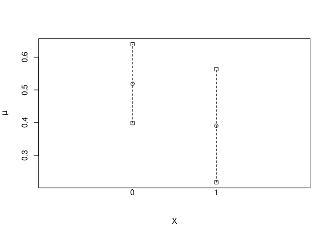

tidy(x)
#>   X   Estimate  Std.Error lower.0.95   upper.0.95   contrast transform
#> 1 0  0.5190639 0.06149960  0.3985269  0.639600881       none  identity
#> 2 1  0.3905311 0.08816362  0.2177336  0.563328623       none  identity
#> 3 0  0.0000000 0.00000000  0.0000000  0.000000000 difference  identity
#> 4 1 -0.1285328 0.06377604 -0.2535315 -0.003534039 difference  identity
#> 5 0  1.0000000 0.00000000  1.0000000  1.000000000      ratio  identity
#> 6 1  0.7523758 0.12604216  0.5053377  0.999413910      ratio  identity

For more detailed examples, see the vignette “Estimation of causal effects using stdReg2”.

Citation

citation("stdReg2")
#> To cite package 'stdReg2' in publications use:
#> 
#>   Sachs M, Sjölander A, Gabriel E, Ohlendorff J (2023). _stdReg2:
#>   Regression Standardization for Causal Inference_. R package version
#>   0.3.0.
#> 
#> A BibTeX entry for LaTeX users is
#> 
#>   @Manual{,
#>     title = {stdReg2: Regression Standardization for Causal Inference},
#>     author = {Michael C Sachs and Arvid Sjölander and Erin E Gabriel and Johan Sebastian Ohlendorff},
#>     year = {2023},
#>     note = {R package version 0.3.0},
#>   }