Introduction and context
Suppose denotes an exposure of interest that takes values 0 or 1. This could represent two different medical treatments, environmental exposures, economic policies, or genetic variants. We will most often use biomedical examples because we are biostatisticians.
We consider the setting where it is of interest to quantify the effect of intervening with on outcome that we will denote . The outcome could represent some numeric value, it could be the presence or absence of a condition, or it could be the time between two events, such as time from cancer diagnosis to death. Let denote the potential outcome if all subjects in the population would hypothetically be exposed to .
To quantify the effect of , we must summarize the distribution of with some statistic. If is dichotomous, it is natural to use , called the risk. If is continuous, the mean is a natural summary statistic . If is a continuous time-to-event, the probability of exceeding a particular value is a reasonable statistic: . In general, denote the summary statistic of choice as . The summary statistic can also be applied to conditional distributions, which we will denote, e.g., .
To quantify the effect of , we must also decide on a contrast to measure the causal effect. The point of the contrast is to compare the chosen summary statistic between the and interventions. Typical choices would be the difference or the ratio . It may also be of interest to quantify and report the summary statistics within each group .
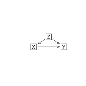
In observational studies, the relationship between and is likely confounded by a set of other variables . This means that the values of the outcome are determined by at least a subset of and the values of the exposure are determined by a subset of . Naively estimating the contrast would lead to biased estimates of the causal effect.
Regression standardization
See Sjölander (2016) and Sjölander (2018) for more details. Suppose that the covariates are sufficient for confounding control. For more information on what constitutes a sufficient adjustment set, see Witte and Didelez (2019). For a given summary statistic , then where the expectation is taken with respect to the population distribution of . This is also known as the g-formula or adjustment formula.
In order to estimate this quantity based on an independent and identically distributed sample , we proceed by
- Specifying and estimating a regression model for given and .
- Use the fitted model to obtain estimates of for . This is done by creating a copy of the observed dataset, replacing the observed with for each individual, and using the fitted model to get predicted values for the copy of the observed data. Denote these predicted values as .
- Average over the empirical distribution of to obtain the estimate
One can do this for each level of and compute the desired contrast. Under the assumptions that 1) is sufficient for confounding control, and 2) the regression model in step 1 is correctly specified, then this estimator is consistent and asymptotically normal.
Improving robustness by modeling the exposure
A doubly-robust estimator is an estimator that is consistent for a given estimand when one or more of the models used in the forming of the estimator is correctly specified for confounding. So far, we only have one model used in our estimator: the outcome model. We will now introduce a model for the exposure, and see how we can combine them. First, some terminology:
Misspecified model - The true generating mechanism is not contained in the possible mechanisms that are possible under the selected model.
Correctly Specified - A model is correctly specified if it is not misspecified.
Correctly specified for confounding - A correctly specified model that contains a sufficient set of confounders.
If we can model , and it is correctly specified and contains all confounders, then we can use that to estimate the probability that each individual received the treatment that they did . Let denote the estimated probability that subject received treatment .
Any consistent estimation method can be used for the outcome and exposure models. As long as either the outcome model or the propensity score model is correctly specified for confounding, then a doubly robust estimator is consistent for the ATE. In this package, for generalized linear models, we use the estimator as described by Gabriel et al. (2024).
Recently, there seems to be a general misconception that combining an adjusted outcome model and a propensity score model always gives a doubly robust estimator. This is not true – it matters how you combine them!
In practice
Here we will use regression standardization to estimate the average
causal effect of the exposure (quitting smoking) in the variable
qsmk on the weight gain outcome in the variable
wt82_71 in the nhefs_complete dataset that
comes with the causaldata package. The data was collected
as part of a project by the National Center for Health Statistics and
the National Institute on Aging in collaboration with other agencies of
the United States Public Health Service. It was designed to investigate
the relationships between clinical, nutritional, and behavioral factors
and subsequent morbidity, mortality, and hospital utilization and
changes in risk factors, functional limitation, and
institutionalization. The dataset includes 1566 individuals and contains
among others the following variables:
- seqn: person id}
- wt82_71: weight gain in kilograms between 1971 and 1982
- qsmk: quit smoking between between 1st questionnaire and 1982, 1 = yes, 0 = no
- sex: 0 = male, 1 = female
- race: 0 = white, 1 = black or other
- age: age in years at baseline
- education: level of education in 1971, 1 = 8th grade or less, 2 = high school dropout, 3 = high school, 4 - dropout, 5 = college or more
- smokeintensity: number of cigarettes smoked per day in 1971
- smokeyrs: number of years smoked
- exercise: level of physical activity in 1971, 0 = much exercise, 1 = moderate exercise, 2 = little or no exercise
- active: level of activity in 1971, 0 = very active, 1 = moderately active, 2 = inactive, 3 = missing
- wt71: weight in kilograms in 1971
- ht: height in centimeters in 1971
nhefs_dat <- causaldata::nhefs_complete
summary(nhefs_dat)
#>       seqn            qsmk            death            yrdth
#>  Min.   :  233   Min.   :0.0000   Min.   :0.0000   Min.   :83.00
#>  1st Qu.:10625   1st Qu.:0.0000   1st Qu.:0.0000   1st Qu.:85.00
#>  Median :20702   Median :0.0000   Median :0.0000   Median :88.00
#>  Mean   :16639   Mean   :0.2573   Mean   :0.1858   Mean   :87.64
#>  3rd Qu.:22771   3rd Qu.:1.0000   3rd Qu.:0.0000   3rd Qu.:90.00
#>  Max.   :25061   Max.   :1.0000   Max.   :1.0000   Max.   :92.00
#>                                                    NA's   :1275
#>      modth            dadth           sbp             dbp         sex
#>  Min.   : 1.000   Min.   : 1.0   Min.   : 87.0   Min.   : 47.00   0:762
#>  1st Qu.: 3.000   1st Qu.: 8.0   1st Qu.:115.0   1st Qu.: 70.00   1:804
#>  Median : 6.000   Median :16.0   Median :126.0   Median : 77.00
#>  Mean   : 6.383   Mean   :16.1   Mean   :128.6   Mean   : 77.74
#>  3rd Qu.:10.000   3rd Qu.:24.5   3rd Qu.:139.0   3rd Qu.: 85.00
#>  Max.   :12.000   Max.   :31.0   Max.   :229.0   Max.   :130.00
#>  NA's   :1271     NA's   :1271   NA's   :29      NA's   :33
#>       age        race         income         marital          school
#>  Min.   :25.00   0:1360   Min.   :11.00   Min.   :2.000   Min.   : 0.00
#>  1st Qu.:33.00   1: 206   1st Qu.:17.00   1st Qu.:2.000   1st Qu.:10.00
#>  Median :43.00            Median :19.00   Median :2.000   Median :12.00
#>  Mean   :43.66            Mean   :17.99   Mean   :2.496   Mean   :11.17
#>  3rd Qu.:53.00            3rd Qu.:20.00   3rd Qu.:2.000   3rd Qu.:12.00
#>  Max.   :74.00            Max.   :22.00   Max.   :8.000   Max.   :17.00
#>                           NA's   :59
#>  education       ht             wt71             wt82           wt82_71
#>  1:291     Min.   :142.9   Min.   : 39.58   Min.   : 35.38   Min.   :-41.280
#>  2:340     1st Qu.:161.8   1st Qu.: 59.53   1st Qu.: 61.69   1st Qu.: -1.478
#>  3:637     Median :168.2   Median : 69.23   Median : 72.12   Median :  2.604
#>  4:121     Mean   :168.7   Mean   : 70.83   Mean   : 73.47   Mean   :  2.638
#>  5:177     3rd Qu.:175.3   3rd Qu.: 79.80   3rd Qu.: 83.46   3rd Qu.:  6.690
#>            Max.   :198.1   Max.   :151.73   Max.   :136.53   Max.   : 48.538
#>
#>    birthplace    smokeintensity  smkintensity82_71    smokeyrs
#>  Min.   : 1.00   Min.   : 1.00   Min.   :-80.000   Min.   : 1.00
#>  1st Qu.:22.00   1st Qu.:10.00   1st Qu.:-10.000   1st Qu.:15.00
#>  Median :34.00   Median :20.00   Median : -1.000   Median :24.00
#>  Mean   :31.67   Mean   :20.53   Mean   : -4.633   Mean   :24.59
#>  3rd Qu.:42.00   3rd Qu.:30.00   3rd Qu.:  1.000   3rd Qu.:33.00
#>  Max.   :56.00   Max.   :80.00   Max.   : 50.000   Max.   :64.00
#>  NA's   :90
#>      asthma            bronch              tb                hf
#>  Min.   :0.00000   Min.   :0.00000   Min.   :0.00000   Min.   :0.000000
#>  1st Qu.:0.00000   1st Qu.:0.00000   1st Qu.:0.00000   1st Qu.:0.000000
#>  Median :0.00000   Median :0.00000   Median :0.00000   Median :0.000000
#>  Mean   :0.04853   Mean   :0.08365   Mean   :0.01341   Mean   :0.005109
#>  3rd Qu.:0.00000   3rd Qu.:0.00000   3rd Qu.:0.00000   3rd Qu.:0.000000
#>  Max.   :1.00000   Max.   :1.00000   Max.   :1.00000   Max.   :1.000000
#>
#>       hbp         pepticulcer        colitis          hepatitis
#>  Min.   :0.000   Min.   :0.0000   Min.   :0.00000   Min.   :0.00000
#>  1st Qu.:0.000   1st Qu.:0.0000   1st Qu.:0.00000   1st Qu.:0.00000
#>  Median :1.000   Median :0.0000   Median :0.00000   Median :0.00000
#>  Mean   :1.059   Mean   :0.1015   Mean   :0.03448   Mean   :0.01788
#>  3rd Qu.:2.000   3rd Qu.:0.0000   3rd Qu.:0.00000   3rd Qu.:0.00000
#>  Max.   :2.000   Max.   :1.0000   Max.   :1.00000   Max.   :1.00000
#>
#>   chroniccough        hayfever          diabetes          polio
#>  Min.   :0.00000   Min.   :0.00000   Min.   :0.0000   Min.   :0.00000
#>  1st Qu.:0.00000   1st Qu.:0.00000   1st Qu.:0.0000   1st Qu.:0.00000
#>  Median :0.00000   Median :0.00000   Median :0.0000   Median :0.00000
#>  Mean   :0.05109   Mean   :0.08621   Mean   :0.9898   Mean   :0.01405
#>  3rd Qu.:0.00000   3rd Qu.:0.00000   3rd Qu.:2.0000   3rd Qu.:0.00000
#>  Max.   :1.00000   Max.   :1.00000   Max.   :2.0000   Max.   :1.00000
#>
#>      tumor          nervousbreak       alcoholpy       alcoholfreq
#>  Min.   :0.00000   Min.   :0.00000   Min.   :0.0000   Min.   :0.000
#>  1st Qu.:0.00000   1st Qu.:0.00000   1st Qu.:1.0000   1st Qu.:1.000
#>  Median :0.00000   Median :0.00000   Median :1.0000   Median :2.000
#>  Mean   :0.02363   Mean   :0.02746   Mean   :0.8787   Mean   :1.913
#>  3rd Qu.:0.00000   3rd Qu.:0.00000   3rd Qu.:1.0000   3rd Qu.:3.000
#>  Max.   :1.00000   Max.   :1.00000   Max.   :2.0000   Max.   :5.000
#>
#>   alcoholtype    alcoholhowmuch        pica          headache
#>  Min.   :1.000   Min.   : 1.000   Min.   :0.000   Min.   :0.0000
#>  1st Qu.:1.000   1st Qu.: 2.000   1st Qu.:0.000   1st Qu.:0.0000
#>  Median :3.000   Median : 2.000   Median :0.000   Median :1.0000
#>  Mean   :2.466   Mean   : 3.293   Mean   :0.986   Mean   :0.6328
#>  3rd Qu.:4.000   3rd Qu.: 4.000   3rd Qu.:2.000   3rd Qu.:1.0000
#>  Max.   :4.000   Max.   :48.000   Max.   :2.000   Max.   :1.0000
#>                  NA's   :397
#>    otherpain        weakheart         allergies           nerves
#>  Min.   :0.0000   Min.   :0.00000   Min.   :0.00000   Min.   :0.000
#>  1st Qu.:0.0000   1st Qu.:0.00000   1st Qu.:0.00000   1st Qu.:0.000
#>  Median :0.0000   Median :0.00000   Median :0.00000   Median :0.000
#>  Mean   :0.2433   Mean   :0.02235   Mean   :0.06322   Mean   :0.145
#>  3rd Qu.:0.0000   3rd Qu.:0.00000   3rd Qu.:0.00000   3rd Qu.:0.000
#>  Max.   :1.0000   Max.   :1.00000   Max.   :1.00000   Max.   :1.000
#>
#>     lackpep            hbpmed       boweltrouble       wtloss
#>  Min.   :0.00000   Min.   :0.000   Min.   :0.000   Min.   :0.00000
#>  1st Qu.:0.00000   1st Qu.:0.000   1st Qu.:0.000   1st Qu.:0.00000
#>  Median :0.00000   Median :1.000   Median :1.000   Median :0.00000
#>  Mean   :0.05045   Mean   :1.015   Mean   :1.046   Mean   :0.02618
#>  3rd Qu.:0.00000   3rd Qu.:2.000   3rd Qu.:2.000   3rd Qu.:0.00000
#>  Max.   :1.00000   Max.   :2.000   Max.   :2.000   Max.   :1.00000
#>
#>    infection     active  exercise  birthcontrol    pregnancies
#>  Min.   :0.000   0:702   0:300    Min.   :0.000   Min.   : 1.000
#>  1st Qu.:0.000   1:715   1:661    1st Qu.:0.000   1st Qu.: 2.000
#>  Median :0.000   2:149   2:605    Median :1.000   Median : 3.000
#>  Mean   :0.145                    Mean   :1.081   Mean   : 3.694
#>  3rd Qu.:0.000                    3rd Qu.:2.000   3rd Qu.: 5.000
#>  Max.   :1.000                    Max.   :2.000   Max.   :15.000
#>                                                   NA's   :866
#>   cholesterol      hightax82         price71         price82
#>  Min.   : 78.0   Min.   :0.0000   Min.   :1.507   Min.   :1.452
#>  1st Qu.:189.0   1st Qu.:0.0000   1st Qu.:2.037   1st Qu.:1.740
#>  Median :216.0   Median :0.0000   Median :2.168   Median :1.815
#>  Mean   :219.9   Mean   :0.1653   Mean   :2.138   Mean   :1.806
#>  3rd Qu.:245.0   3rd Qu.:0.0000   3rd Qu.:2.242   3rd Qu.:1.868
#>  Max.   :416.0   Max.   :1.0000   Max.   :2.693   Max.   :2.103
#>  NA's   :16      NA's   :90       NA's   :90      NA's   :90
#>      tax71            tax82          price71_82         tax71_82
#>  Min.   :0.5249   Min.   :0.2200   Min.   :-0.2027   Min.   :0.03599
#>  1st Qu.:0.9449   1st Qu.:0.4399   1st Qu.: 0.2010   1st Qu.:0.46100
#>  Median :1.0498   Median :0.5060   Median : 0.3360   Median :0.54395
#>  Mean   :1.0580   Mean   :0.5058   Mean   : 0.3324   Mean   :0.55220
#>  3rd Qu.:1.1548   3rd Qu.:0.5719   3rd Qu.: 0.4438   3rd Qu.:0.62195
#>  Max.   :1.5225   Max.   :0.7479   Max.   : 0.6121   Max.   :0.88440
#>  NA's   :90       NA's   :90       NA's   :90        NA's   :90
#>        id            censored     older
#>  Min.   :   1.0   Min.   :0   Min.   :0.0000
#>  1st Qu.: 414.2   1st Qu.:0   1st Qu.:0.0000
#>  Median : 824.5   Median :0   Median :0.0000
#>  Mean   : 821.0   Mean   :0   Mean   :0.2989
#>  3rd Qu.:1228.8   3rd Qu.:0   3rd Qu.:1.0000
#>  Max.   :1629.0   Max.   :0   Max.   :1.0000
#>
We will assume that the set of confounders in includes sex, race, age, education, number of cigarettes smoked per year, the number of years smoked, level of physical activity, and baseline weight in 1971. This equivalent to assuming that the counterfactual weight gain is independent of the exposure conditional on these variables. In other words, we are assuming the following directed acyclic graph:
For the specific forms of the conditional expectations required in the outcome we assume a linear regression model with both linear and quadratic forms of the continuous covariates. We can fit this as
m <- glm(wt82_71 ~ qsmk + sex + race + age + I(age^2) +
        as.factor(education) + smokeintensity + I(smokeintensity^2) +
        smokeyrs + I(smokeyrs^2) + as.factor(exercise) + as.factor(active) +
          wt71 + I(wt71^2),
        data = nhefs_dat)
summary(m)
#>
#> Call:
#> glm(formula = wt82_71 ~ qsmk + sex + race + age + I(age^2) +
#>     as.factor(education) + smokeintensity + I(smokeintensity^2) +
#>     smokeyrs + I(smokeyrs^2) + as.factor(exercise) + as.factor(active) +
#>     wt71 + I(wt71^2), data = nhefs_dat)
#>
#> Coefficients:
#>                         Estimate Std. Error t value Pr(>|t|)
#> (Intercept)           -1.6586176  4.3137734  -0.384 0.700666
#> qsmk                   3.4626218  0.4384543   7.897 5.36e-15 ***
#> sex1                  -1.4650496  0.4683410  -3.128 0.001792 **
#> race1                  0.5864117  0.5816949   1.008 0.313560
#> age                    0.3626624  0.1633431   2.220 0.026546 *
#> I(age^2)              -0.0061377  0.0017263  -3.555 0.000389 ***
#> as.factor(education)2  0.8185263  0.6067815   1.349 0.177546
#> as.factor(education)3  0.5715004  0.5561211   1.028 0.304273
#> as.factor(education)4  1.5085173  0.8323778   1.812 0.070134 .
#> as.factor(education)5 -0.1708264  0.7413289  -0.230 0.817786
#> smokeintensity         0.0651533  0.0503115   1.295 0.195514
#> I(smokeintensity^2)   -0.0010468  0.0009373  -1.117 0.264261
#> smokeyrs               0.1333931  0.0917319   1.454 0.146104
#> I(smokeyrs^2)         -0.0018270  0.0015438  -1.183 0.236818
#> as.factor(exercise)1   0.3206824  0.5349616   0.599 0.548961
#> as.factor(exercise)2   0.3628786  0.5589557   0.649 0.516300
#> as.factor(active)1    -0.9429574  0.4100208  -2.300 0.021593 *
#> as.factor(active)2    -0.2580374  0.6847219  -0.377 0.706337
#> wt71                   0.0373642  0.0831658   0.449 0.653297
#> I(wt71^2)             -0.0009158  0.0005235  -1.749 0.080426 .
#> ---
#> Signif. codes:  0 '***' 0.001 '**' 0.01 '*' 0.05 '.' 0.1 ' ' 1
#>
#> (Dispersion parameter for gaussian family taken to be 53.59474)
#>
#>     Null deviance: 97176  on 1565  degrees of freedom
#> Residual deviance: 82857  on 1546  degrees of freedom
#> AIC: 10701
#>
#> Number of Fisher Scoring iterations: 2
To perform regression standardization to estimate the causal effect
we use standardize_glm. We must specify the same outcome
regression model as a formula, provide the data, describe which values
of the exposure we wish to estimate the counterfactual means, specify
which contrasts we want, and specify the reference level for the
contrasts. The following command estimates that model and we obtain the
group-wise estimates, the difference, and the ratio.
m2 <- standardize_glm(wt82_71 ~ qsmk + sex + race + age + I(age^2) +
               as.factor(education) + smokeintensity + I(smokeintensity^2) +
               smokeyrs + I(smokeyrs^2) + as.factor(exercise) + as.factor(active) +
               wt71 + I(wt71^2),
            data = nhefs_dat,
            values = list(qsmk = c(0,1)),
            contrasts = c("difference", "ratio"),
            reference = 0)

m2
#> Outcome formula: wt82_71 ~ qsmk + sex + race + age + I(age^2) + as.factor(education) +
#>     smokeintensity + I(smokeintensity^2) + smokeyrs + I(smokeyrs^2) +
#>     as.factor(exercise) + as.factor(active) + wt71 + I(wt71^2)
#> Outcome family: gaussian
#> Outcome link function: identity
#> Exposure:  qsmk
#>
#> Tables:
#>   qsmk Estimate Std.Error lower.0.95 upper.0.95
#> 1    0     1.75     0.256       1.25       2.25
#> 2    1     5.21     0.356       4.51       5.91
#>
#> Reference level:  qsmk = 0
#> Contrast:  difference
#>   qsmk Estimate Std.Error lower.0.95 upper.0.95
#> 1    0     0.00     0.000       0.00       0.00
#> 2    1     3.46     0.418       2.64       4.28
#>
#> Reference level:  qsmk = 0
#> Contrast:  ratio
#>   qsmk Estimate Std.Error lower.0.95 upper.0.95
#> 1    0     1.00     0.000       1.00       1.00
#> 2    1     2.98     0.463       2.07       3.89

plot(m2)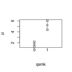
plot(m2, contrast = "difference", reference = 0)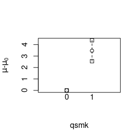
The output from the model shows the estimated potential outcome means in each exposure level, the difference and ratio thereof, and the associated standard error estimates, confidence intervals, and p-values. Inference is done using the sandwich method for variance calculation. Under the assumptions that the outcome model is correctly specified and contains all confounders, these are consistent estimates of the causal effects of interest. We can also get plots of the effects by using the plot function.
To obtain the estimates and inference for the different contrasts as
a tidy data frame, suitable for saving as a data table or using in
downstream analyses or reports, we provide the tidy
function:
(tidy(m2) -> tidy_m2) |> print()
#>   qsmk Estimate Std.Error lower.0.95 upper.0.95   contrast transform
#> 1    0 1.747216 0.2556332   1.246184   2.248248       none  identity
#> 2    1 5.209838 0.3563820   4.511342   5.908334       none  identity
#> 3    0 0.000000 0.0000000   0.000000   0.000000 difference  identity
#> 4    1 3.462622 0.4176304   2.644081   4.281162 difference  identity
#> 5    0 1.000000 0.0000000   1.000000   1.000000      ratio  identity
#> 6    1 2.981793 0.4630392   2.074253   3.889334      ratio  identity
To obtain doubly robust inference we use the following command. Note that we now specify a model for the exposure, the propensity score model.
m2_dr <- standardize_glm_dr(formula_outcome = wt82_71 ~ qsmk + sex + race + age + I(age^2) +
               as.factor(education) + smokeintensity + I(smokeintensity^2) +
               smokeyrs + I(smokeyrs^2) + as.factor(exercise) + as.factor(active) +
               wt71 + I(wt71^2),
               formula_exposure = qsmk ~ sex + race + age + I(age^2) +
                as.factor(education) + smokeintensity + I(smokeintensity^2) +
                smokeyrs + I(smokeyrs^2) + as.factor(exercise) + as.factor(active) +
                wt71 + I(wt71^2),
            data = nhefs_dat,
            values = list(qsmk = c(0,1)),
            contrast = c("difference", "ratio"),
            reference = 0)

m2_dr
#> Doubly robust estimator with:
#>
#> Exposure formula: qsmk ~ sex + race + age + I(age^2) + as.factor(education) + smokeintensity +
#>     I(smokeintensity^2) + smokeyrs + I(smokeyrs^2) + as.factor(exercise) +
#>     as.factor(active) + wt71 + I(wt71^2)
#> Exposure link function: logit
#> Outcome formula: wt82_71 ~ qsmk + sex + race + age + I(age^2) + as.factor(education) +
#>     smokeintensity + I(smokeintensity^2) + smokeyrs + I(smokeyrs^2) +
#>     as.factor(exercise) + as.factor(active) + wt71 + I(wt71^2)
#> Outcome family: gaussian
#> Outcome link function: identity
#> Exposure:  qsmk
#>
#> Tables:
#>   qsmk Estimate Std.Error lower.0.95 upper.0.95
#> 1    0     1.76     0.218       1.34       2.19
#> 2    1     5.19     0.438       4.33       6.04
#>
#> Reference level:  qsmk = 0
#> Contrast:  difference
#>   qsmk Estimate Std.Error lower.0.95 upper.0.95
#> 1    0     0.00      0.00       0.00       0.00
#> 2    1     3.42      0.48       2.48       4.37
#>
#> Reference level:  qsmk = 0
#> Contrast:  ratio
#>   qsmk Estimate Std.Error lower.0.95 upper.0.95
#> 1    0     1.00     0.000        1.0       1.00
#> 2    1     2.94     0.431        2.1       3.79

(tidy(m2_dr) -> tidy_m2_dr) |> print()
#>   qsmk Estimate Std.Error lower.0.95 upper.0.95   contrast transform
#> 1    0 1.762981 0.2176810   1.336334   2.189628       none  identity
#> 2    1 5.186772 0.4378466   4.328609   6.044936       none  identity
#> 3    0 0.000000 0.0000000   0.000000   0.000000 difference  identity
#> 4    1 3.423792 0.4804026   2.482220   4.365363 difference  identity
#> 5    0 1.000000 0.0000000   1.000000   1.000000      ratio  identity
#> 6    1 2.942047 0.4310190   2.097265   3.786829      ratio  identity
Based on these results, we can report that the estimated effect of smoking on average weight change as measured by the difference in potential outcome means is 3.46 (2.64 to 4.28) and as measured by the ratio of potential outcome means is 2.98 (2.07 to 3.89). Using the doubly-robust estimation method, we obtain similarly 3.42 (2.48 to 4.37) and as measured by the ratio of potential outcome means is 2.94 (2.10 to 3.79). In particular, if we believe that the necessary assumptions are valid, we can conclude that smoking causes an increase in weight which the numeric summaries indicate that smoking increases the weight change over 11 years by about 3.5 pounds (additive scale) or smoking increases the weight change over 11 years by a multiplicative factor of about 3.
The doubly-robust method requires specification of an exposure model
in addition to the specification of the outcome model. Both of these
estimated models can be accessed and inspected by looking at the
fit_outcome and fit_exposure elements of the
return object:
m2_dr$res$fit_outcome
#>
#> Call:  fit_glm(formula = formula_outcome, family = family_outcome, data = data,
#>     response = "outcome", weights = weights)
#>
#> Coefficients:
#>           (Intercept)                   qsmk                   sex1
#>            -1.931e+00              3.424e+00             -1.989e+00
#>                 race1                    age               I(age^2)
#>             4.707e-01              6.207e-01             -8.678e-03
#> as.factor(education)2  as.factor(education)3  as.factor(education)4
#>             1.935e+00              8.366e-01              2.564e+00
#> as.factor(education)5         smokeintensity    I(smokeintensity^2)
#>             8.339e-01              1.130e-01             -2.240e-03
#>              smokeyrs          I(smokeyrs^2)   as.factor(exercise)1
#>             1.034e-01             -1.473e-03              7.865e-01
#>  as.factor(exercise)2     as.factor(active)1     as.factor(active)2
#>             1.231e+00             -8.251e-01             -4.576e-01
#>                  wt71              I(wt71^2)
#>            -1.221e-01              8.616e-06
#>
#> Degrees of Freedom: 1565 Total (i.e. Null);  1546 Residual
#> Null Deviance:       212700
#> Residual Deviance: 175100    AIC: 11030
m2_dr$res$fit_exposure
#>
#> Call:  fit_glm(formula = formula_exposure, family = family_exposure,
#>     data = data, response = "exposure", weights = weights)
#>
#> Coefficients:
#>           (Intercept)                   sex1                  race1
#>            -2.2425191             -0.5274782             -0.8392636
#>                   age               I(age^2)  as.factor(education)2
#>             0.1212052             -0.0008246             -0.0287755
#> as.factor(education)3  as.factor(education)4  as.factor(education)5
#>             0.0864318              0.0636010              0.4759606
#>        smokeintensity    I(smokeintensity^2)               smokeyrs
#>            -0.0772704              0.0010451             -0.0735966
#>         I(smokeyrs^2)   as.factor(exercise)1   as.factor(exercise)2
#>             0.0008441              0.3548405              0.3957040
#>    as.factor(active)1     as.factor(active)2                   wt71
#>             0.0319445              0.1767840             -0.0152357
#>             I(wt71^2)
#>             0.0001352
#>
#> Degrees of Freedom: 1565 Total (i.e. Null);  1547 Residual
#> Null Deviance:       1786
#> Residual Deviance: 1677  AIC: 1715
This is useful when we want to inspect the distribution of the propensity scores by exposure status. This is an important thing to check in practice, we are looking for any practical violations of the positivity assumption.
hist(m2_dr$res$fit_exposure$fitted[nhefs_dat$qsmk == 0],
    xlim = c(0, 1), main = "qsmk = 0", xlab = "estimated propensity")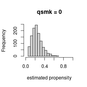
hist(m2_dr$res$fit_exposure$fitted[nhefs_dat$qsmk == 1],
    xlim = c(0, 1), main = "qsmk = 1", xlab = "estimated propensity")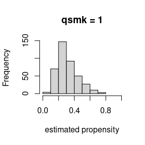
Other outcome types
The function standardize_glm and its doubly-robust
counterpart standardize_glm_dr support any outcome variable
type the can be used with glm. This includes binary, count,
and more. Just like in glm, we specify the model we would
like to use for the outcome by specifying the family
argument of standardize_glm or the
family_outcome argument of standardize_glm_dr.
By default this is "gaussian" which corresponds to linear
regression. For a binary outcome we might like to use
"binomial" which corresponds to logistic regression. Let us
see how it works using the a binary outcome that we create by
dichotomizing the weight change at 0.
nhefs_dat$gained_weight <- 1.0 * (nhefs_dat$wt82_71 > 0)
m3 <- standardize_glm(gained_weight ~ qsmk + sex + race + age + I(age^2) +
               as.factor(education) + smokeintensity + I(smokeintensity^2) +
               smokeyrs + I(smokeyrs^2) + as.factor(exercise) + as.factor(active) +
               wt71 + I(wt71^2),
            data = nhefs_dat,
            family = "binomial",
            values = list(qsmk = c(0,1)),
            contrasts = c("difference", "ratio"),
            reference = 0)

m3
#> Outcome formula: gained_weight ~ qsmk + sex + race + age + I(age^2) + as.factor(education) +
#>     smokeintensity + I(smokeintensity^2) + smokeyrs + I(smokeyrs^2) +
#>     as.factor(exercise) + as.factor(active) + wt71 + I(wt71^2)
#> Outcome family: quasibinomial
#> Outcome link function: logit
#> Exposure:  qsmk
#>
#> Tables:
#>   qsmk Estimate Std.Error lower.0.95 upper.0.95
#> 1    0    0.639    0.0141      0.611      0.666
#> 2    1    0.772    0.0203      0.732      0.811
#>
#> Reference level:  qsmk = 0
#> Contrast:  difference
#>   qsmk Estimate Std.Error lower.0.95 upper.0.95
#> 1    0    0.000    0.0000     0.0000      0.000
#> 2    1    0.133    0.0247     0.0846      0.181
#>
#> Reference level:  qsmk = 0
#> Contrast:  ratio
#>   qsmk Estimate Std.Error lower.0.95 upper.0.95
#> 1    0     1.00    0.0000       1.00       1.00
#> 2    1     1.21    0.0414       1.13       1.29
Here we interpret the estimates in terms of probabilities, or the risk of gaining weight over 11 years. In particular, smoking causes a 13% additive increase in the risk of gaining weight, or a 1.2 fold multiplicative increase in the risk of gaining weight. With binary outcomes, we can use transformations to get different contrasts, and also to improve the performance of the ratio contrast. By using the log transformation combined with the difference contrast, our estimates become the log risk ratios. We can exponential them to get the risk ratios, but often it is better to construct confidence intervals of ratios on the log scale and back transform.
m3_log <- standardize_glm(gained_weight ~ qsmk + sex + race + age + I(age^2) +
               as.factor(education) + smokeintensity + I(smokeintensity^2) +
               smokeyrs + I(smokeyrs^2) + as.factor(exercise) + as.factor(active) +
               wt71 + I(wt71^2),
            data = nhefs_dat,
            family = "binomial",
            values = list(qsmk = c(0,1)),
            contrasts = c("difference"),
            transforms = c("log"),
            reference = 0)
m3_log
#> Outcome formula: gained_weight ~ qsmk + sex + race + age + I(age^2) + as.factor(education) +
#>     smokeintensity + I(smokeintensity^2) + smokeyrs + I(smokeyrs^2) +
#>     as.factor(exercise) + as.factor(active) + wt71 + I(wt71^2)
#> Outcome family: quasibinomial
#> Outcome link function: logit
#> Exposure:  qsmk
#>
#> Tables:
#> Transform:
#>   qsmk Estimate Std.Error lower.0.95 upper.0.95
#> 1    0   -0.448    0.0221     -0.492     -0.405
#> 2    1   -0.259    0.0264     -0.311     -0.208
#>
#> Transform:
#> Reference level:  qsmk = 0
#> Contrast:  difference
#>   qsmk Estimate Std.Error lower.0.95 upper.0.95
#> 1    0    0.000    0.0000      0.000      0.000
#> 2    1    0.189    0.0343      0.122      0.256
The estimates reported in the table are log risk ratios, which we now back transform by exponentiating and compare to the ratios estimated previously.
tm3_log <- tidy(m3_log)
tm3_log$rr <- exp(tm3_log$Estimate)
tm3_log$rr.lower <- exp(tm3_log$lower.0.95)
tm3_log$rr.upper <- exp(tm3_log$upper.0.95)

subset(tm3_log, contrast == "difference" & qsmk == 1)
#>   qsmk  Estimate  Std.Error lower.0.95 upper.0.95   contrast transform       rr
#> 4    1 0.1890909 0.03427325  0.1219166  0.2562653 difference       log 1.208151
#>   rr.lower rr.upper
#> 4  1.12966 1.292095
m3
#> Outcome formula: gained_weight ~ qsmk + sex + race + age + I(age^2) + as.factor(education) +
#>     smokeintensity + I(smokeintensity^2) + smokeyrs + I(smokeyrs^2) +
#>     as.factor(exercise) + as.factor(active) + wt71 + I(wt71^2)
#> Outcome family: quasibinomial
#> Outcome link function: logit
#> Exposure:  qsmk
#>
#> Tables:
#>   qsmk Estimate Std.Error lower.0.95 upper.0.95
#> 1    0    0.639    0.0141      0.611      0.666
#> 2    1    0.772    0.0203      0.732      0.811
#>
#> Reference level:  qsmk = 0
#> Contrast:  difference
#>   qsmk Estimate Std.Error lower.0.95 upper.0.95
#> 1    0    0.000    0.0000     0.0000      0.000
#> 2    1    0.133    0.0247     0.0846      0.181
#>
#> Reference level:  qsmk = 0
#> Contrast:  ratio
#>   qsmk Estimate Std.Error lower.0.95 upper.0.95
#> 1    0     1.00    0.0000       1.00       1.00
#> 2    1     1.21    0.0414       1.13       1.29
In this case, the estimates and inference using transformation are nearly identical to those without transformation.
Other available transformations include the odds, and logit (log odds). These can be used to estimate causal odds ratios, untransformed and transformed, respectively.
m3_odds <- standardize_glm(gained_weight ~ qsmk + sex + race + age + I(age^2) +
               as.factor(education) + smokeintensity + I(smokeintensity^2) +
               smokeyrs + I(smokeyrs^2) + as.factor(exercise) + as.factor(active) +
               wt71 + I(wt71^2),
            data = nhefs_dat,
            family = "binomial",
            values = list(qsmk = c(0,1)),
            contrasts = c("ratio"),
            transforms = c("odds"),
            reference = 0)
m3_odds
#> Outcome formula: gained_weight ~ qsmk + sex + race + age + I(age^2) + as.factor(education) +
#>     smokeintensity + I(smokeintensity^2) + smokeyrs + I(smokeyrs^2) +
#>     as.factor(exercise) + as.factor(active) + wt71 + I(wt71^2)
#> Outcome family: quasibinomial
#> Outcome link function: logit
#> Exposure:  qsmk
#>
#> Tables:
#> Transform:
#>   qsmk Estimate Std.Error lower.0.95 upper.0.95
#> 1    0     1.77     0.108       1.55       1.98
#> 2    1     3.38     0.390       2.61       4.14
#>
#> Transform:
#> Reference level:  qsmk = 0
#> Contrast:  ratio
#>   qsmk Estimate Std.Error lower.0.95 upper.0.95
#> 1    0     1.00     0.000       1.00        1.0
#> 2    1     1.91     0.249       1.42        2.4

m3_logit <- standardize_glm(gained_weight ~ qsmk + sex + race + age + I(age^2) +
               as.factor(education) + smokeintensity + I(smokeintensity^2) +
               smokeyrs + I(smokeyrs^2) + as.factor(exercise) + as.factor(active) +
               wt71 + I(wt71^2),
            data = nhefs_dat,
            family = "binomial",
            values = list(qsmk = c(0,1)),
            contrasts = c("difference"),
            transforms = c("logit"),
            reference = 0)
m3_logit
#> Outcome formula: gained_weight ~ qsmk + sex + race + age + I(age^2) + as.factor(education) +
#>     smokeintensity + I(smokeintensity^2) + smokeyrs + I(smokeyrs^2) +
#>     as.factor(exercise) + as.factor(active) + wt71 + I(wt71^2)
#> Outcome family: quasibinomial
#> Outcome link function: logit
#> Exposure:  qsmk
#>
#> Tables:
#> Transform:
#>   qsmk Estimate Std.Error lower.0.95 upper.0.95
#> 1    0    0.569    0.0612      0.449      0.689
#> 2    1    1.217    0.1154      0.991      1.443
#>
#> Transform:
#> Reference level:  qsmk = 0
#> Contrast:  difference
#>   qsmk Estimate Std.Error lower.0.95 upper.0.95
#> 1    0    0.000      0.00      0.000      0.000
#> 2    1    0.648      0.13      0.393      0.903

m3_logOR <- tidy(m3_logit) |>
  subset(contrast == "difference" & qsmk == 1)

sprintf("%.2f (%.2f to %.2f)", exp(m3_logOR$Estimate),
        exp(m3_logOR$lower.0.95), exp(m3_logOR$upper.0.95))
#> [1] "1.91 (1.48 to 2.47)"
In this case the estimate is identical, but the confidence interval is slightly different because it is symmetric on the odds ratio scale in the first case, and symmetric on the log odds ratio scale in the transformed case.